


Home » Knowledge platform » Documents and studies » OSR Tools » Remote sensing
In a broad sense, these are the means by which information is captured through remote observation of the territory, and the techniques and knowledge used to interpret this information. Specifically, it applies to the collection of electromagnetic radiation from sensors located on mobile platforms (satellites) and the interpretation of this data.
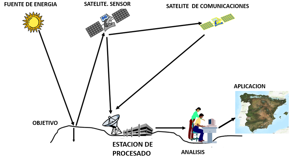
Figure 1. General scheme for remote sensing data acquisition and processing.
Satellites collect energy reflected from the Earth's surface at different wavelengths (depending on the sensors the satellite carries). The electromagnetic spectrum has a wide range of wavelengths.
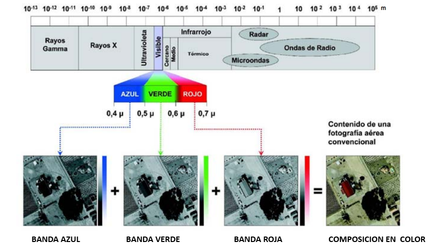
Figure 2. Electromagnetic spectrum.
Each wavelength provides suitable information for studying various characteristics of the Earth's surface. For example, visible radiation (0.4 to 0.7 nanometers) provides information on the photosynthetic activity of plants; near-infrared (NIR, 0.7 to 2.5 nanometers) allows for the characterization of vegetation growth; thermal infrared (TIR, 2.5 to 20 nanometers) characterizes the water status of vegetation; and radar wavelengths (0.5 cm to 1 m) provide interpretable information for characterizing surface soil moisture.
Satellites collect surface reflectivity data (for each pixel of the terrain) and store it in multiple bands (one band per wavelength). This information can be represented in two ways:
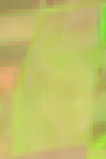
Visualization of a combination corresponding to the NIR, Red, and Green bands (called false color, since it assigns the NIR band data to the red color channel, the red band data to the green channel, and the green band data to the blue channel). In this combination, vigorous vegetation is shown in shades of red.
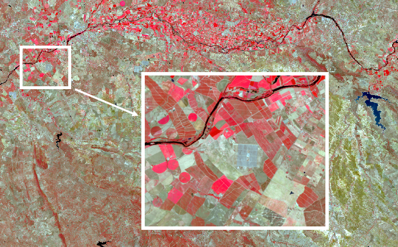
Figure 3. Example of a Sentinel image from June 2, 2023 in northern Badajoz (false color).
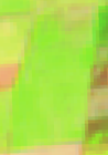
Another example that is more similar to how the human eye generates color corresponds to the combination of red, green, and blue bands (called natural color), in which vigorous vegetation is seen in shades of green.
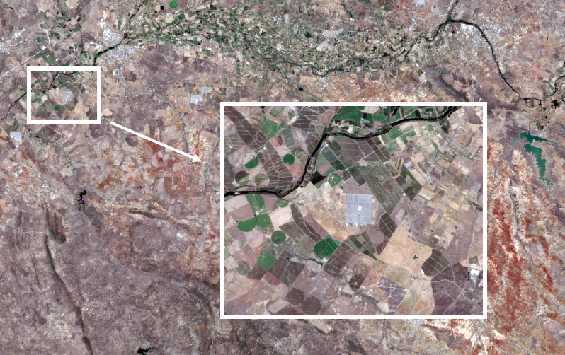
Figure 4. Example of a Sentinel image from June 2, 2023, in northern Badajoz (true color).
The graphical representation of reflected energy as a function of wavelength for a pixel (or group of pixels) is called a spectral signature. It is characteristic of each type of land cover; for example, in vegetation, chlorophyll absorbs radiation in the red channel and reflects it sharply in the infrared.
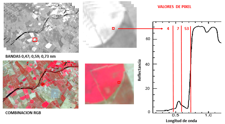
Figure 5. Numerical value of reflectance in a pixel in 3 bands.
The spectral signature of vegetation from data from a satellite like Landsat TM, which has 7 bands (and therefore collects data at 7 wavelengths), is shown as a simplified line compared to the continuous representation typical of other satellites that work with many more bands:
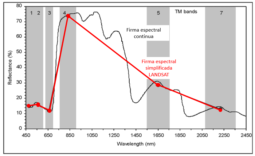
Figure 6. Spectral signature of a plant cover.
Below is a summary table with the characteristics of a selection of satellites with open data and historical archives, with multiple applications in agriculture and the environment.
| SATELLITE / SENSOR | IMAGE WIDTH (Km) | NUMBER OF BANDS | PIXEL SIZE | DAYS BETWEEN IMAGES | FILE START DATE |
|---|---|---|---|---|---|
| MODIS Terra-Aqua | 2.330 | 36 bands (in wave length: A,V, R, CRI, MRI, T) | 250 m (R, IR) 500 m (A, V, IRC) 1Km (A, V, R, IRC, IRM, T) | Daily | Since: 1999 Terra 2002 Aqua |
| Landsat 5 TM | 190 | 7 bands (A, V, R, CRI, MRI, T) | 30m Multi 120 m T | 16 | 1984-2013 |
| Landsat 7 EMT+ | 190 | 1 PAM band 8-band Multi | 15 m pan 30m Multi 60 m T | 16 | Since 1999 |
| Landsat 8 OLI | 190 | 1 PAM band 8-band Multi | 15m pan30m Multi 100 m T | 16 | Since 2013 |
| Sentinel-2 MSI | 290 Tiles 100x100 | 13 Multi-Bands | 10 m (A, V, IRC) 20 m (BR, IRC, IRM) 60 m (A, IRC, IRM) | 5 | From: 2015 S2A 2017 S2B |
| Sentinel-1 C-SAR | 250 | Dual: VV+VH,HH+HV Simpl: HH, VV | 5×20 m | 6 | From: 2014 S1A 2016 S1B |
Figure 7. Satellites with open archive images.
They are the result of mathematical operations performed between the values of the spectral bands of the starting images, in order to obtain synthetic images that highlight the information of interest about the land cover, mitigating problems such as differences in lighting or noise in the starting images.
Typically, indices are applied to multi-time series of images to analyze the evolution of different land cover types over time, whether to observe the phenology of different crops, the state of forest stands, the flooded area in wetlands, the evolution of areas affected by fires, and so on.
Some of the most commonly used indices are, for example:
He NDVI (Normalized Difference Vegetation Index (from Rouse et al., 1973). It is an index correlated with vegetative activity. Its values range from -1 to 1, with higher values corresponding to vigorous vegetation. Its main limitation is that it tends to become saturated when vegetation is very dense. It is calculated using the following banding relationship.
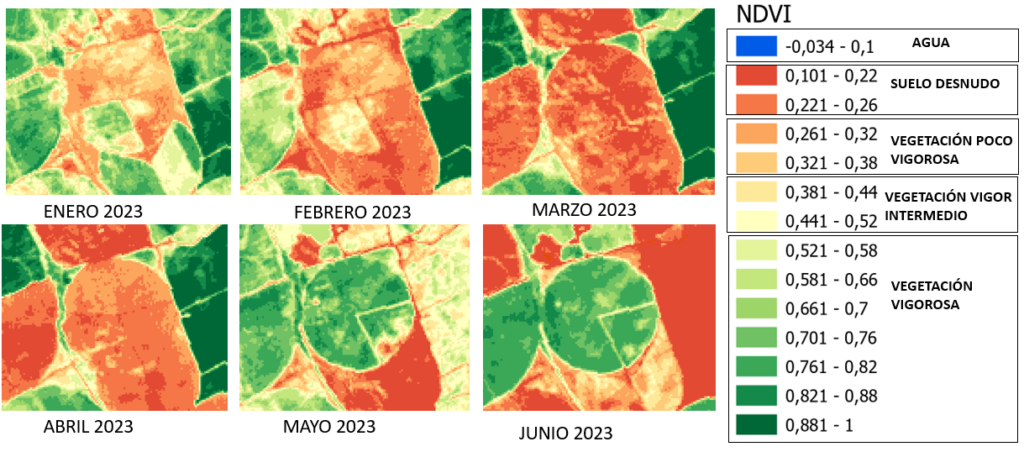
Figure 8. Visualization of monthly NDVI in corn pivot.
He SAVI (Soil-Adjusted Vegetation Index. (Huete, 1988). It is an index equivalent to NDVI that introduces the parameter L, which allows adjusting the contribution of soil reflectivity. L varies between 0 and 1, with the value 0.5 used for intermediate vegetation densities (1 for low densities and 0.25 for high densities).
He NDWI (Normalized Difference Water Index. (Gao, 1996). It is a normalized index used to determine water content and water stress in vegetation. Values range from -1 to 1, with higher values indicating greater water content. It is calculated using the band ratio:
Remote sensing data is available at varying intervals depending on the satellite (for example, Landsat every 16 days, Sentinel-2 every 5 days). This data allows for low-cost crop monitoring throughout its entire development cycle. Studies can be conducted at the plot level or across large areas. Inputting this data into various agronomic models provides results that can be used to manage crop needs (for example, in calculating irrigation, fertilizer, and pesticide requirements).
| April 6 | June 13 | June 25 | August 27 | October 8 |
 |  |  |  |  |
| Sowing | Development vegetative | Bloom | Maturation | Harvest |
|---|---|---|---|---|
 |  |  |  | 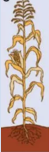 |
| 0 – 7 days | 7 – 50 days 2 months | 50 – 53 days | 53 – 110 days | 110 – 120 days |
| April | April – June | June – August | September – October |
Figure 9. Visualization of Landsat images in correspondence with phenological stages of the corn crop.
Statistical treatment of the information provided by vegetation indices allows the identification of problems throughout the development of the crop, for example, by comparing, on each date, the values of the indices in the study area with the average values that would be expected.
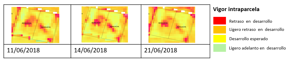
Figure 10. Alerts of vigor problems in plots obtained from NDVI on different dates.
Using spectral signatures with a multiband image from a specific date, or with images from multiple dates, allows pixels with similar characteristics to be grouped into classes. The algorithms used to identify similar pixels are highly varied.
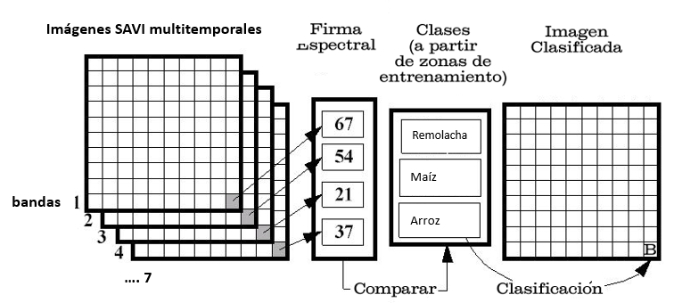
Figure 11. Schematic representation of the image classification process.
Specifically developing the case of the use of remote sensing data in agronomic models such as those used to calculate water needs in crops, we see that there are multiple models for calculating crop evapotranspiration (ETc):
Most are approximations to the surface energy balance that uses remote sensing data and meteorological data, among other data sets, as inputs.
Among them, the Allen model allows deriving the FAO crop evaporation coefficient (Kc) that intervenes in the calculation of Evapotranspiration from NDVI, in herbaceous crops, with the expression: Kc = 1.25 x NDVI + 0.1 (Allen et al., 2008)
From this Kc and the potential evapotranspiration (ETo) obtained from weather stations, the actual crop evapotranspiration (ETc) can be calculated. This data can be used:
At the farmer level: to plan irrigation (the combination of information provided by satellite images, with moisture probes and weather data prediction allows irrigation to be requested at the most suitable times)
At the level of irrigation management bodies to make forecasts/management of water consumption throughout the irrigation season.
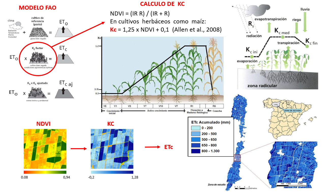
Figure 12. Calculation scheme of Kc in herbaceous plants with Allen model and derived ET.
Another example of the use of remote sensing is the input of NDVI into agronomic models to derive yield values as outlined below in the Biomass Estimation Model based on light use.
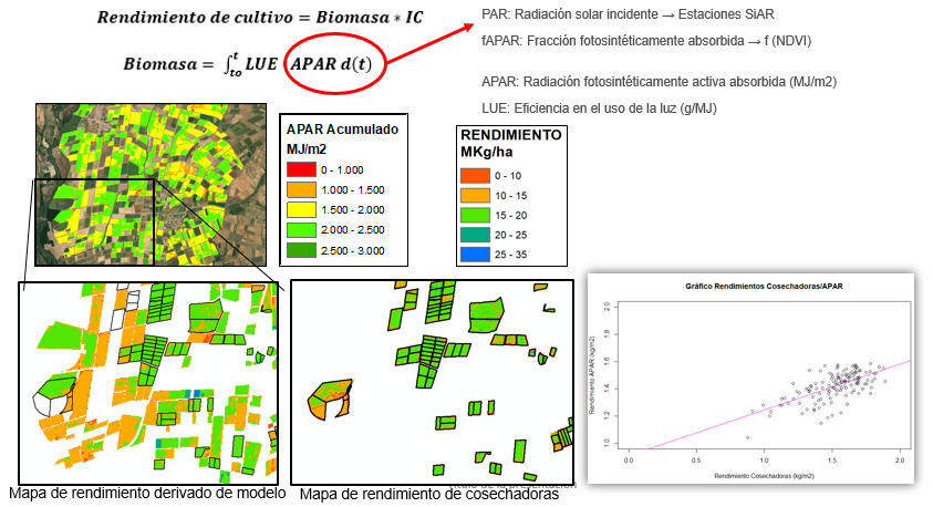
Figure 13. Calculation of biomass and derived crop yield in maize.
In this model, the NDVI allows estimating the radiation absorbed by the plants throughout their vegetative cycle, and this translates into a quantification of the biomass produced and a derived yield by adjusting various parameters involved in the model.
Other possible uses of remote sensing include automatic detection of changes, monitoring of floods, fires…
Technical support to irrigation communities
Collaboration with irrigators from the Porma, Payuelos, and Páramo communities in León. Since the 2017 season, various remote sensing products (false-color and natural-color image visualization, vegetation indices, Kcs of plots, and vegetation vigor alert images) have been offered and made available to irrigation communities and irrigation managers through a viewer.
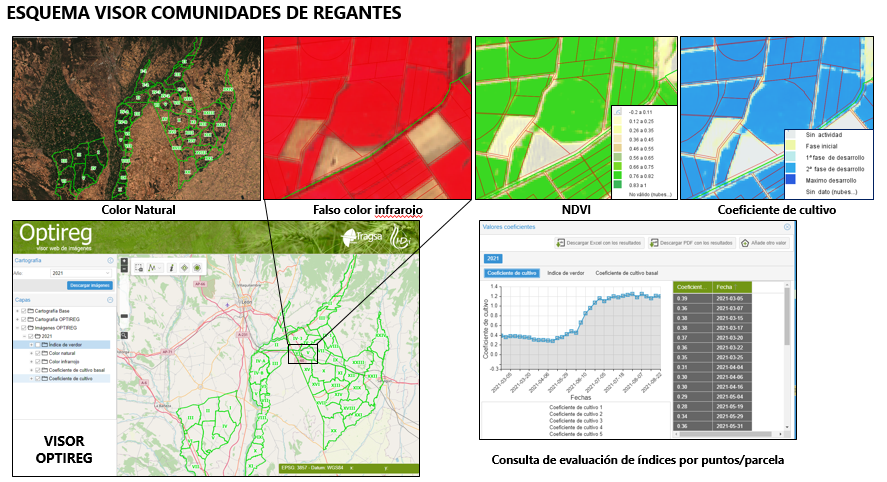
Figure 14. OPTIREG viewer scheme for irrigation communities in León.
Calculation of water needs in the SIAR
Since the 2016 campaign, the calculation of irrigation water needs at the national level has been carried out using as starting data, among others, the series of Landsat 8 and Sentinel 2 images available in each campaign and generating a series of intermediate products such as the map of land use in irrigation, the monthly and annual ETc maps and the monthly and annual irrigation needs maps.
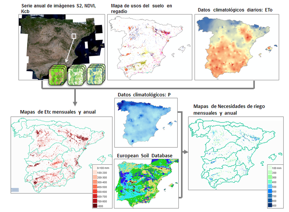
Figure 15. Outline of the starting data used in the SIAR project and the products generated.
Monitoring of herbaceous crops in the CAP aid system
Since 1994, partial statistical controls of crops have been carried out on the ground, based on medium and high resolution satellite images, to support the CAP aid system.
Since 2019, the availability of open data with sufficient resolution and coverage from the Copernicus program allows for 100% monitoring of the national surface using new technologies for accessing and processing satellite data in the cloud.
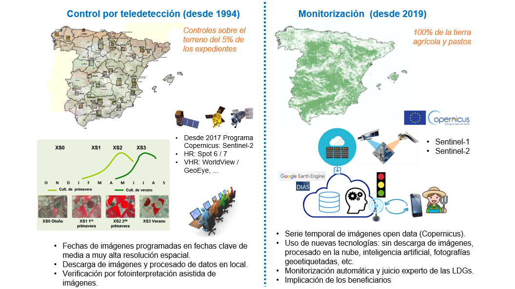
Figure 16. Outline of the starting data used in the SIAR project and the products generated.